17YJunction.C

Introduction to tutorial 17

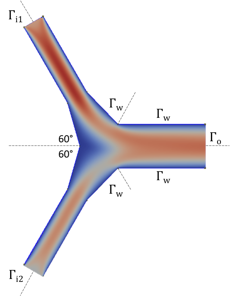
In this tutorial, we contruct a reduced order model for a Y-junction flow problem. The Y-junction consists of two inlets and one outlet channel whose time-dependent inlet boundary conditions are controlled. The angle between each inlet and the horizontal axis is 60 degrees. The length of the channels is 2 m. The two inlets, \(\Gamma_{i1}\) and \(\Gamma_{i2}\), have a width of 0.5 m, while the outlet, \(\Gamma_{o}\), has a width of 1 m. The kinematic viscosity is equal to \(\nu\) = 0.01 m \(^2\)/s and the flow is considered laminar. As initial conditions the steady state solution, obtained with the simpleFOAM-solver, for a velocity magnitude of 1 m/s at both inlets is chosen. In this tutorial, new values of the velocity magnitude of the flow at the inlets are imposed in the reduced order model with either an iterative penalty method or a lifting function method. The reduced order model is constructed using Galerkin projection approach together with an exploitation of a pressure Poisson equation during the projection stage.

The following image depicts a sketch of the geometry of the two-dimensional Y-junction.

A detailed look into the code

In this section we explain the main steps necessary to construct the tutorial N°17.

The necessary header files

First of all let's have a look at the header files that need to be included and what they are responsible for.

The header files of ITHACA-FV necessary for this tutorial are: <unsteadyNS.H> for the full order unsteady NS problem, <ITHACAPOD.H> for the POD decomposition, <reducedUnsteadyNS.H> for the construction of the reduced order problem, and finally <ITHACAstream.H> for some ITHACA input-output operations.

#include "unsteadyNS.H"
#include "ITHACAPOD.H"
#include "ReducedUnsteadyNS.H"
#include "ITHACAstream.H"

Definition of the tutorial17 class

We define the tutorial17 class as a child of the unsteadyNS class.

class tutorial17: public unsteadyNS
{
    public:
        explicit tutorial17(int argc, char* argv[])
            :
            unsteadyNS(argc, argv),
            U(_U()),
            p(_p())
        {}
 
        // Fields To Perform
        volVectorField& U;
        volScalarField& p;

Inside the tutorial17 class we define the offlineSolve method according to the specific problem that needs to be solved. If the offline solve has been previously performed then the method just reads the existing snapshots from the Offline directory. Otherwise it performs the offline solve.

        void offlineSolve()
        {
            List<scalar> mu_now(1);
            volVectorField U0 = U;
            volScalarField P0 = p;
 
            if (offline)
            {
                ITHACAstream::read_fields(Ufield, U, "./ITHACAoutput/Offline/");
                ITHACAstream::read_fields(Pfield, p, "./ITHACAoutput/Offline/");
            }
            else
            {
                U = U0;
                p = P0;
                mu_now[0] = mu(0, 0);
                truthSolve(mu_now);
            }
        }

We also define a liftSolve method, which will be needed to construct the lifting functions if the lifting function method is used:

        void liftSolve(Eigen::MatrixXd BCs)
        {
            for (label k = 0; k < inletPatch.rows(); k++)
            {
                Time& runTime = _runTime();
                surfaceScalarField& phi = _phi();
                fvMesh& mesh = _mesh();
                volScalarField p = _p();
                volVectorField U = _U();
                IOMRFZoneList& MRF = _MRF();
                label BCind = inletPatch(k, 0);
                volVectorField Ulift("Ulift" + name(k), U);
                instantList Times = runTime.times();
                runTime.setTime(Times[1], 1);
                pisoControl potentialFlow(mesh, "potentialFlow");
                Info << "Solving a lifting Problem" << endl;
                Vector<double> v1(0, 0, 0);
                v1[0] = BCs(0, k);
                v1[1] = BCs(1, k);
                Vector<double> v0(0, 0, 0);
 
                for (label j = 0; j < U.boundaryField().size(); j++)
                {
                    if (j == BCind)
                    {
                        assignBC(Ulift, j, v1);
                    }
                    else if (U.boundaryField()[BCind].type() == "fixedValue")
                    {
                        assignBC(Ulift, j, v0);
                    }
                    else
                    {
                    }
 
                    assignIF(Ulift, v0);
                    phi = linearInterpolate(Ulift) & mesh.Sf();
                }
 
                Info << "Constructing velocity potential field Phi\n" << endl;
                volScalarField Phi
                (
                    IOobject
                    (
                        "Phi",
                        runTime.timeName(),
                        mesh,
                        IOobject::READ_IF_PRESENT,
                        IOobject::NO_WRITE
                    ),
                    mesh,
                    dimensionedScalar("Phi", dimLength * dimVelocity, 0),
                    p.boundaryField().types()
                );
                label PhiRefCell = 0;
                scalar PhiRefValue = 0;
                setRefCell
                (
                    Phi,
                    potentialFlow.dict(),
                    PhiRefCell,
                    PhiRefValue
                );
                mesh.setFluxRequired(Phi.name());
                runTime.functionObjects().start();
                MRF.makeRelative(phi);
                adjustPhi(phi, Ulift, p);
 
                while (potentialFlow.correctNonOrthogonal())
                {
                    fvScalarMatrix PhiEqn
                    (
                        fvm::laplacian(dimensionedScalar("1", dimless, 1), Phi)
                        ==
                        fvc::div(phi)
                    );
                    PhiEqn.setReference(PhiRefCell, PhiRefValue);
                    PhiEqn.solve();
 
                    if (potentialFlow.finalNonOrthogonalIter())
                    {
                        phi -= PhiEqn.flux();
                    }
                }
 
                MRF.makeAbsolute(phi);
                Info << "Continuity error = "
                     << mag(fvc::div(phi))().weightedAverage(mesh.V()).value()
                     << endl;
                Ulift = fvc::reconstruct(phi);
                Ulift.correctBoundaryConditions();
                Info << "Interpolated velocity error = "
                     << (sqrt(sum(sqr((fvc::interpolate(U) & mesh.Sf()) - phi)))
                         / sum(mesh.magSf())).value()
                     << endl;
                Ulift.write();
                volVectorField Uzero
                (
                    IOobject
                    (
                        "Uzero",
                        U.time().timeName(),
                        U.mesh(),
                        IOobject::NO_READ,
                        IOobject::AUTO_WRITE
                    ),
                    U.mesh(),
                    dimensionedVector("zero", U.dimensions(), vector::zero)
                );
                volVectorField Uliftx("Uliftx" + name(k), Uzero);
                Uliftx.replace(0, Ulift.component(0));
                Uliftx.write();
                liftfield.append((Uliftx).clone());
                volVectorField Ulifty("Ulifty" + name(k), Uzero);
                Ulifty.replace(1, Ulift.component(1));
                Ulifty.write();
                liftfield.append((Ulifty).clone());
            }
        }

Definition of the main function

In this section we show the definition of the main function. First we construct the object "example" of type tutorial17:

    tutorial17 example(argc, argv);

Next, we specify the name of the file that contains the values at the boundary for the full order solver for each time step. The inlet velocity magnitude of, alternately, inlet 1 or 2 is increased or decreased linearly over time between 1.0 m/s to 0.5 m/s.

    word par_offline_BC("./timeBCoff");

The input file only contains the boundary values at inlet 1 and 2 in the x-direction and y-direction. We are storing these values in an matrix together with zero velocity in the z-direction since it is required to specify the velocity in the x,y and z direction even though the problem is two-dimensional.

    Eigen::MatrixXd timeBCoff2D = ITHACAstream::readMatrix(par_offline_BC);
    Eigen::MatrixXd timeBCoff3D = Eigen::MatrixXd::Zero(6, timeBCoff2D.cols());
    timeBCoff3D.row(0) = timeBCoff2D.row(0);
    timeBCoff3D.row(1) = timeBCoff2D.row(1);
    timeBCoff3D.row(3) = timeBCoff2D.row(2);
    timeBCoff3D.row(4) = timeBCoff2D.row(3);
    example.timeBCoff = timeBCoff3D;

We also load the new inlet velocities for the reduced order solver from a text file and store the values in a matrix.

    Eigen::MatrixXd par_on_BC;
    word par_online_BC("./timeBCon");
    par_on_BC = ITHACAstream::readMatrix(par_online_BC);

Then we parse the ITHACAdict file to determine the number of modes to be written out and also the ones to be used for projection of the velocity and pressure:

    ITHACAparameters* para = ITHACAparameters::getInstance(example._mesh(),
                             example._runTime());
    int NmodesUout = para->ITHACAdict->lookupOrDefault<int>("NmodesUout", 15);
    int NmodesPout = para->ITHACAdict->lookupOrDefault<int>("NmodesPout", 15);
    int NmodesSUPout = para->ITHACAdict->lookupOrDefault<int>("NmodesSUPout", 15);
    int NmodesUproj = para->ITHACAdict->lookupOrDefault<int>("NmodesUproj", 10);
    int NmodesPproj = para->ITHACAdict->lookupOrDefault<int>("NmodesPproj", 10);
    int NmodesSUPproj = para->ITHACAdict->lookupOrDefault<int>("NmodesSUPproj", 10);

we note that a default value can be assigned in case the parser did not find the corresponding string in the ITHACAdict file.

In our implementation, the viscocity needs to be defined by specifying that Nparameters=1, Nsamples=1, and the parameter ranges from 0.01 to 0.01 equispaced, i.e.

    example.Pnumber = 1;
 
    example.Tnumber = 1;
    example.setParameters();
    // Set the parameter ranges
    example.mu_range(0, 0) = 0.01;
    example.mu_range(0, 1) = 0.01;
    // Generate equispaced samples inside the parameter range
    example.genEquiPar();

After that we set the inlet boundaries where we have the non homogeneous BC

    example.inletIndex.resize(4, 2); // rows: total number of patches
    example.inletIndex(0, 0) = 1;  // Patch inlet 1
    example.inletIndex(0, 1) = 0;  // Patch inlet 1: x-direction
    example.inletIndex(1, 0) = 1;  // Patch inlet 1: y-direction
    example.inletIndex(1, 1) = 1;  // Patch inlet 2
    example.inletIndex(2, 0) = 2;  // Patch inlet 2: x-direction
    example.inletIndex(2, 1) = 0;  // Patch inlet 2: y-direction
    example.inletIndex(3, 0) = 2;  // Patch inlet 2: x-direction
    example.inletIndex(3, 1) = 1;  // Patch inlet 2: y-direction

as well as the patch number of inlet 1 and the patch number of inlet 2.

    example.inletPatch.resize(2, 1);
    example.inletPatch(0, 0) = example.inletIndex(0, 0);  // Patch inlet 1
    example.inletPatch(1, 0) = example.inletIndex(2, 0);  // Patch inlet 2

We set the parameters for the time integration, so as to simulate 12.0 seconds of simulation time, with a step size = 0.0005 seconds, and the data are dumped every 0.03 seconds, i.e.

    example.startTime = 0;
    example.finalTime = 12;
    example.timeStep = 0.0005;
    example.writeEvery = 0.03;

Now we are ready to perform the offline stage:

    example.offlineSolve();

After that, the modes for the velocity and pressure are obtained. The lifting function method requires the velocity modes to be homogeneous. Therefore we differentiate here between the lifting function method and the penalty method. Which bcMethod to be used can be specified in the ITHACAdict file.

In the case of the lifting function method, we specify first a unit value onto the inlet patches in the x- and y-direction

    if (example.bcMethod == "lift")
    {
        // Search the lift function
        Eigen::MatrixXd BCs;
        BCs.resize(2, 2);
        BCs(0, 0) = 1;  // Patch inlet 1
        BCs(1, 0) = -1;  // Patch inlet 2
        BCs(0, 1) = 1;  // Patch inlet 1
        BCs(1, 1) = 1;  // Patch inlet 2

Then we solve for the lifting functions; one lifting function for each inlet boundary condition and direction

        example.liftSolve(BCs);

The lifting functions are normalized

        ITHACAutilities::normalizeFields(example.liftfield);

and the velocity snapshots are homogenized by subtracting the normalized lifting functions from the velocity snapshots.

        example.computeLift(example.Ufield, example.liftfield, example.Uomfield);

Finally, we obtain the homogeneous velocity modes

        ITHACAPOD::getModes(example.Uomfield, example.Umodes, example._U().name(),
                            example.podex, 0, 0,
                            NmodesUout);

and the pressure modes.

        ITHACAPOD::getModes(example.Pfield, example.Pmodes, example._p().name(),
                            example.podex, 0, 0,
                            NmodesPout);
    }

If the penalty method is used, the velocity and pressure modes are computed as follows

    else if (example.bcMethod == "penalty")
    {
        // Perform a POD decomposition for velocity and pressure
        ITHACAPOD::getModes(example.Ufield, example.Umodes, example._U().name(),
                            example.podex, 0, 0,
                            NmodesUout);
        ITHACAPOD::getModes(example.Pfield, example.Pmodes, example._p().name(),
                            example.podex, 0, 0,
                            NmodesPout);
    }

Then the projection onto the POD modes is performed using the Pressure Poisson Equation (PPE) approach.

    example.projectPPE("./Matrices", NmodesUproj, NmodesPproj, NmodesSUPproj);

Now that we obtained all the necessary information from the POD decomposition and the reduced matrices, we are ready to construct the dynamical system for the reduced order model (ROM). We proceed by constructing the object "reduced" of type reducedUnsteadyNS:

    reducedUnsteadyNS reduced(example);

And then we can use the constructed ROM to perform the online procedure, from which we can simulate the problem for new values of the inlet velocities that vary linearly over time. We are keeping the time stepping the same as for the offline stage, but the ROM simulation (online stage) is performed for a longer time period.

    reduced.nu = 0.01;
    reduced.tstart = 0;
    reduced.finalTime = 18;
    reduced.dt = 0.0005;
    reduced.storeEvery = 0.0005;
    reduced.exportEvery = 0.03;

We have to specify a new value for the inlet velocities, which were already loaded from a text file

    Eigen::MatrixXd vel_now = par_on_BC;

If the penalty method is used, we also have to set the parameters for the iterative penalty method to determine a suitable penalty factor

    if (example.bcMethod == "penalty")
    {
        // Set values of the iterative penalty method
        reduced.maxIterPenalty = 100;
        reduced.tolerancePenalty = 1e-5;
        reduced.timeStepPenalty = 5;
        // Set initial quess for penalty factors
        reduced.tauIter = Eigen::MatrixXd::Zero(4, 1);
        reduced.tauIter <<  1e-6, 1e-6, 1e-6, 1e-6;
        // Solve for the penalty factors with the iterative solver
        reduced.tauU = reduced.penalty_PPE(vel_now, reduced.tauIter);
    }

and then the online solve is performed.

    reduced.solveOnline_PPE(vel_now);

Finally the ROM solution is reconstructed. In the case the solution should be exported and exported, put true instead of false in the function:

    reduced.reconstruct(false, "./ITHACAoutput/Reconstruction/");

The plain program

Here there's the plain code

/*---------------------------------------------------------------------------*\
     ██╗████████╗██╗  ██╗ █████╗  ██████╗ █████╗       ███████╗██╗   ██╗
     ██║╚══██╔══╝██║  ██║██╔══██╗██╔════╝██╔══██╗      ██╔════╝██║   ██║
     ██║   ██║   ███████║███████║██║     ███████║█████╗█████╗  ██║   ██║
     ██║   ██║   ██╔══██║██╔══██║██║     ██╔══██║╚════╝██╔══╝  ╚██╗ ██╔╝
     ██║   ██║   ██║  ██║██║  ██║╚██████╗██║  ██║      ██║      ╚████╔╝
     ╚═╝   ╚═╝   ╚═╝  ╚═╝╚═╝  ╚═╝ ╚═════╝╚═╝  ╚═╝      ╚═╝       ╚═══╝
 
 * In real Time Highly Advanced Computational Applications for Finite Volumes
 * Copyright (C) 2021 by the ITHACA-FV authors
-------------------------------------------------------------------------------
License
    This file is part of ITHACA-FV
    ITHACA-FV is free software: you can redistribute it and/or modify
    it under the terms of the GNU Lesser General Public License as published by
    the Free Software Foundation, either version 3 of the License, or
    (at your option) any later version.
    ITHACA-FV is distributed in the hope that it will be useful,
    but WITHOUT ANY WARRANTY; without even the implied warranty of
    MERCHANTABILITY or FITNESS FOR A PARTICULAR PURPOSE. See the
    GNU Lesser General Public License for more details.
    You should have received a copy of the GNU Lesser General Public License
    along with ITHACA-FV. If not, see <http://www.gnu.org/licenses/>.
Description
    Example of an unsteady NS Reduction Problem with time-dependent boundary
    conditions.
SourceFiles
    17YJunction.C
\*---------------------------------------------------------------------------*/
#include "unsteadyNS.H"
#include "ITHACAPOD.H"
#include "ReducedUnsteadyNS.H"
#include "ITHACAstream.H"
#include <chrono>
#include <math.h>
#include <iomanip>
 
class tutorial17: public unsteadyNS
{
    public:
        explicit tutorial17(int argc, char* argv[])
            :
            unsteadyNS(argc, argv),
            U(_U()),
            p(_p())
        {}
 
        // Fields To Perform
        volVectorField& U;
        volScalarField& p;
 
        void offlineSolve()
        {
            List<scalar> mu_now(1);
            volVectorField U0 = U;
            volScalarField P0 = p;
 
            if (offline)
            {
                ITHACAstream::read_fields(Ufield, U, "./ITHACAoutput/Offline/");
                ITHACAstream::read_fields(Pfield, p, "./ITHACAoutput/Offline/");
            }
            else
            {
                U = U0;
                p = P0;
                mu_now[0] = mu(0, 0);
                truthSolve(mu_now);
            }
        }
 
        // Method to compute the lifting functions for this tutorial
        void liftSolve(Eigen::MatrixXd BCs)
        {
            for (label k = 0; k < inletPatch.rows(); k++)
            {
                Time& runTime = _runTime();
                surfaceScalarField& phi = _phi();
                fvMesh& mesh = _mesh();
                volScalarField p = _p();
                volVectorField U = _U();
                IOMRFZoneList& MRF = _MRF();
                label BCind = inletPatch(k, 0);
                volVectorField Ulift("Ulift" + name(k), U);
                instantList Times = runTime.times();
                runTime.setTime(Times[1], 1);
                pisoControl potentialFlow(mesh, "potentialFlow");
                Info << "Solving a lifting Problem" << endl;
                Vector<double> v1(0, 0, 0);
                v1[0] = BCs(0, k);
                v1[1] = BCs(1, k);
                Vector<double> v0(0, 0, 0);
 
                for (label j = 0; j < U.boundaryField().size(); j++)
                {
                    if (j == BCind)
                    {
                        assignBC(Ulift, j, v1);
                    }
                    else if (U.boundaryField()[BCind].type() == "fixedValue")
                    {
                        assignBC(Ulift, j, v0);
                    }
                    else
                    {
                    }
 
                    assignIF(Ulift, v0);
                    phi = linearInterpolate(Ulift) & mesh.Sf();
                }
 
                Info << "Constructing velocity potential field Phi\n" << endl;
                volScalarField Phi
                (
                    IOobject
                    (
                        "Phi",
                        runTime.timeName(),
                        mesh,
                        IOobject::READ_IF_PRESENT,
                        IOobject::NO_WRITE
                    ),
                    mesh,
                    dimensionedScalar("Phi", dimLength * dimVelocity, 0),
                    p.boundaryField().types()
                );
                label PhiRefCell = 0;
                scalar PhiRefValue = 0;
                setRefCell
                (
                    Phi,
                    potentialFlow.dict(),
                    PhiRefCell,
                    PhiRefValue
                );
                mesh.setFluxRequired(Phi.name());
                runTime.functionObjects().start();
                MRF.makeRelative(phi);
                adjustPhi(phi, Ulift, p);
 
                while (potentialFlow.correctNonOrthogonal())
                {
                    fvScalarMatrix PhiEqn
                    (
                        fvm::laplacian(dimensionedScalar("1", dimless, 1), Phi)
                        ==
                        fvc::div(phi)
                    );
                    PhiEqn.setReference(PhiRefCell, PhiRefValue);
                    PhiEqn.solve();
 
                    if (potentialFlow.finalNonOrthogonalIter())
                    {
                        phi -= PhiEqn.flux();
                    }
                }
 
                MRF.makeAbsolute(phi);
                Info << "Continuity error = "
                     << mag(fvc::div(phi))().weightedAverage(mesh.V()).value()
                     << endl;
                Ulift = fvc::reconstruct(phi);
                Ulift.correctBoundaryConditions();
                Info << "Interpolated velocity error = "
                     << (sqrt(sum(sqr((fvc::interpolate(U) & mesh.Sf()) - phi)))
                         / sum(mesh.magSf())).value()
                     << endl;
                Ulift.write();
                volVectorField Uzero
                (
                    IOobject
                    (
                        "Uzero",
                        U.time().timeName(),
                        U.mesh(),
                        IOobject::NO_READ,
                        IOobject::AUTO_WRITE
                    ),
                    U.mesh(),
                    dimensionedVector("zero", U.dimensions(), vector::zero)
                );
                volVectorField Uliftx("Uliftx" + name(k), Uzero);
                Uliftx.replace(0, Ulift.component(0));
                Uliftx.write();
                liftfield.append((Uliftx).clone());
                volVectorField Ulifty("Ulifty" + name(k), Uzero);
                Ulifty.replace(1, Ulift.component(1));
                Ulifty.write();
                liftfield.append((Ulifty).clone());
            }
        }
 
};
 
/*---------------------------------------------------------------------------*\
                               Starting the MAIN
\*---------------------------------------------------------------------------*/
int main(int argc, char* argv[])
{
    // Construct the tutorial17 object
    tutorial17 example(argc, argv);
    // the offline samples for the boundary conditions
    word par_offline_BC("./timeBCoff");
    // Convert boundary values x-direction and y-direction to x,y,z
    Eigen::MatrixXd timeBCoff2D = ITHACAstream::readMatrix(par_offline_BC);
    Eigen::MatrixXd timeBCoff3D = Eigen::MatrixXd::Zero(6, timeBCoff2D.cols());
    timeBCoff3D.row(0) = timeBCoff2D.row(0);
    timeBCoff3D.row(1) = timeBCoff2D.row(1);
    timeBCoff3D.row(3) = timeBCoff2D.row(2);
    timeBCoff3D.row(4) = timeBCoff2D.row(3);
    example.timeBCoff = timeBCoff3D;
    Eigen::MatrixXd par_on_BC;
    word par_online_BC("./timeBCon");
    par_on_BC = ITHACAstream::readMatrix(par_online_BC);
    // Read parameters from ITHACAdict file
    ITHACAparameters* para = ITHACAparameters::getInstance(example._mesh(),
                             example._runTime());
    int NmodesUout = para->ITHACAdict->lookupOrDefault<int>("NmodesUout", 15);
    int NmodesPout = para->ITHACAdict->lookupOrDefault<int>("NmodesPout", 15);
    int NmodesSUPout = para->ITHACAdict->lookupOrDefault<int>("NmodesSUPout", 15);
    int NmodesUproj = para->ITHACAdict->lookupOrDefault<int>("NmodesUproj", 10);
    int NmodesPproj = para->ITHACAdict->lookupOrDefault<int>("NmodesPproj", 10);
    int NmodesSUPproj = para->ITHACAdict->lookupOrDefault<int>("NmodesSUPproj", 10);
    int NmodesOut = para->ITHACAdict->lookupOrDefault<int>("NmodesOut", 20);
    example.Pnumber = 1;
    example.Tnumber = 1;
    example.setParameters();
    // Set the parameter ranges
    example.mu_range(0, 0) = 0.01;
    example.mu_range(0, 1) = 0.01;
    // Generate equispaced samples inside the parameter range
    example.genEquiPar();
    // Set the inlet boundaries where we have non homogeneous boundary conditions
    example.inletIndex.resize(4, 2); // rows: total number of patches
    example.inletIndex(0, 0) = 1;  // Patch inlet 1
    example.inletIndex(0, 1) = 0;  // Patch inlet 1: x-direction
    example.inletIndex(1, 0) = 1;  // Patch inlet 1: y-direction
    example.inletIndex(1, 1) = 1;  // Patch inlet 2
    example.inletIndex(2, 0) = 2;  // Patch inlet 2: x-direction
    example.inletIndex(2, 1) = 0;  // Patch inlet 2: y-direction
    example.inletIndex(3, 0) = 2;  // Patch inlet 2: x-direction
    example.inletIndex(3, 1) = 1;  // Patch inlet 2: y-direction
    example.inletPatch.resize(2, 1);
    example.inletPatch(0, 0) = example.inletIndex(0, 0);  // Patch inlet 1
    example.inletPatch(1, 0) = example.inletIndex(2, 0);  // Patch inlet 2
    // Time parameters
    example.startTime = 0;
    example.finalTime = 12;
    example.timeStep = 0.0005;
    example.writeEvery = 0.03;
    // Perform The Offline Solve;
    example.offlineSolve();
 
    // Perform POD
    if (example.bcMethod == "lift")
    {
        // Search the lift function
        Eigen::MatrixXd BCs;
        BCs.resize(2, 2);
        BCs(0, 0) = 1;  // Patch inlet 1
        BCs(1, 0) = -1;  // Patch inlet 2
        BCs(0, 1) = 1;  // Patch inlet 1
        BCs(1, 1) = 1;  // Patch inlet 2
        example.liftSolve(BCs);
        // Normalize the lifting function
        ITHACAutilities::normalizeFields(example.liftfield);
        // Create homogeneous basis functions for velocity
        example.computeLift(example.Ufield, example.liftfield, example.Uomfield);
        // Perform a POD decomposition for velocity and pressure
        ITHACAPOD::getModes(example.Uomfield, example.Umodes, example._U().name(),
                            example.podex, 0, 0,
                            NmodesUout);
        ITHACAPOD::getModes(example.Pfield, example.Pmodes, example._p().name(),
                            example.podex, 0, 0,
                            NmodesPout);
    }
    else if (example.bcMethod == "penalty")
    {
        // Perform a POD decomposition for velocity and pressure
        ITHACAPOD::getModes(example.Ufield, example.Umodes, example._U().name(),
                            example.podex, 0, 0,
                            NmodesUout);
        ITHACAPOD::getModes(example.Pfield, example.Pmodes, example._p().name(),
                            example.podex, 0, 0,
                            NmodesPout);
    }
 
    // Reduced Matrices
    example.projectPPE("./Matrices", NmodesUproj, NmodesPproj, NmodesSUPproj);
    reducedUnsteadyNS reduced(example);
    // Set values of the online phase
    reduced.nu = 0.01;
    reduced.tstart = 0;
    reduced.finalTime = 18;
    reduced.dt = 0.0005;
    reduced.storeEvery = 0.0005;
    reduced.exportEvery = 0.03;
    // Set values velocity boundary conditions of the online phase
    Eigen::MatrixXd vel_now = par_on_BC;
 
    if (example.bcMethod == "penalty")
    {
        // Set values of the iterative penalty method
        reduced.maxIterPenalty = 100;
        reduced.tolerancePenalty = 1e-5;
        reduced.timeStepPenalty = 5;
        // Set initial quess for penalty factors
        reduced.tauIter = Eigen::MatrixXd::Zero(4, 1);
        reduced.tauIter <<  1e-6, 1e-6, 1e-6, 1e-6;
        // Solve for the penalty factors with the iterative solver
        reduced.tauU = reduced.penalty_PPE(vel_now, reduced.tauIter);
    }
 
    // Set the online temperature BC and solve reduced model
    reduced.solveOnline_PPE(vel_now);
    reduced.reconstruct(false, "./ITHACAoutput/Reconstruction/");
    exit(0);
}