Introduction to tutorial 19
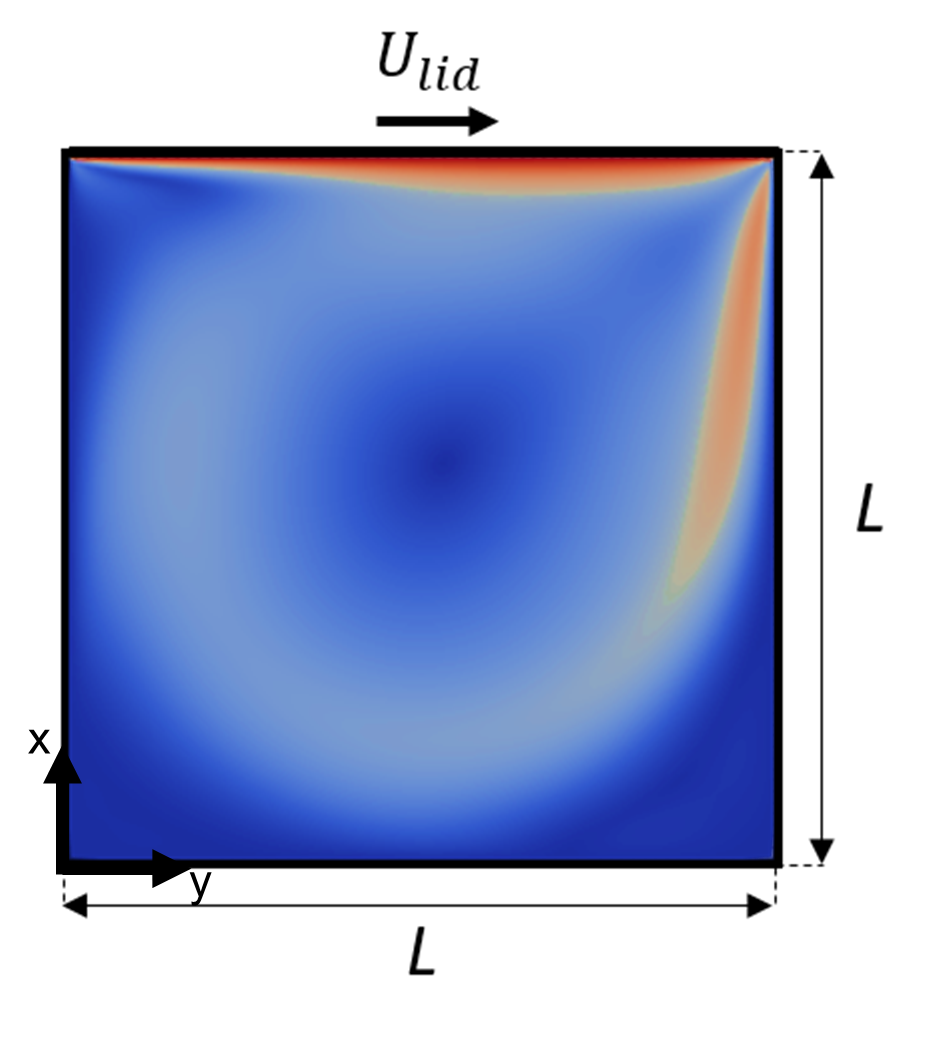
In this tutorial we contruct a reduced order model for the classical lid driven cavity benchmark, which is a closed flow problem. The length of the two-dimensional square cavity is \(L\) = 1.0 m. A (64 \(\times\) 64) structured mesh with quadrilateral cells is constructed on the domain. A tangential uniform velocity \(U_{lid}\) = 1.0 m/s is prescribed at the top wall and non-slip conditions are applied to the other walls.
The following image depicts a sketch of the geometry of the two-dimensional lid driven cavity problem.
The Reynolds number based on the velocity of the lid and the cavity characteristic length is 100 and the flow is considered laminar. The initial condition for the cell-centered velocity is a zero field. A full order simulation is performed for a constant time step of 0.005 s and for a total simulation time of 1.0 s in the offline stage.
In this tutorial, we employ explicit time integration methods at the full order and the reduced order level. We derive the reduced order model via the projection of the fully discrete system.
A detailed look into the code
In this section we explain the main steps necessary to construct the tutorial N°19
The necessary header files
First of all let's have a look at the header files that need to be included and what they are responsible for.
The header files of ITHACA-FV necessary for this tutorial are: <UnsteadyNSExplicit.H> for the full order unsteady NS problem discretized in time using Forward Euler, <ITHACAPOD.H> for the POD decomposition, <ReducedUnsteadyNSExplicit.H> for the construction of the reduced order problem, and finally <ITHACAstream.H> for some ITHACA input-output operations.
19UnsteadyNSExplicit.C
\*---------------------------------------------------------------------------*/
Header file of the ITHACAPOD class.
Header file of the ITHACAstream class, it contains the implementation of several methods for input ou...
Header file of the ReducedUnsteadyNSExplicit class.
Header file of the UnsteadyNSExplicit class.
Definition of the tutorial19 class
We define the tutorial19 class as a child of the UnsteadyNSExplicit class. The constructor is defined with members that are the fields need to be manipulated during the resolution of the full order problem using either a inconsistent flux method or a consistent flux method. Such fields are also initialized with the same initial conditions in the solver.
Implementation of a parametrized full order unsteady NS problem and preparation of the the reduced ...
{
public:
:
{}
UnsteadyNSExplicit()
Construct Null.
autoPtr< volVectorField > _U
Velocity field.
tutorial19(int argc, char *argv[])
Inside the tutorial19 class we define the offlineSolve method according to the specific problem that needs to be solved. If the offline solve has been previously performed then the method just reads the existing velocity and pressure snapshots from the Offline directory. Otherwise it performs the offline solve. If the inconsistent flux method is selected, the snapshots of the fluxes (phi) are also read. The fluxMethod needs to be defined in the ITHACAdict file (inconsistent or consistent).
{
Vector<double> inl(1, 0, 0);
List<scalar> mu_now(1);
{
{
}
}
else
bool offline
Boolean variable, it is 1 if the Offline phase has already been computed, else 0.
PtrList< volScalarField > Pfield
List of pointers used to form the pressure snapshots matrix.
PtrList< volVectorField > Ufield
List of pointers used to form the velocity snapshots matrix.
PtrList< surfaceScalarField > Phifield
List of pointers used to form the flux snapshots matrix.
word fluxMethod
Flux Method.
void read_fields(PtrList< GeometricField< Type, PatchField, GeoMesh > > &Lfield, word Name, fileName casename, int first_snap, int n_snap)
Function to read a list of fields from the name of the field and casename.
{
for (label
i = 0;
i <
mu.cols();
i++)
{
}
Eigen::MatrixXd mu
Row matrix of parameters.
void truthSolve()
Perform a TruthSolve.
}
}
Definition of the main function
In this section we show the definition of the main function. First we construct the object "example" of type tutorial19:
Then we parse the ITHACAdict file to determine the number of modes to be written out and also the ones to be used for projection of the velocity and pressure. The discretize-then-project approach does not need any supremizer modes:
Class for the definition of some general parameters, the parameters must be defined from the file ITH...
static ITHACAparameters * getInstance()
Gets an instance of ITHACAparameters, to be used if the instance is already existing.
example._runTime());
int NmodesUout =
para->ITHACAdict->lookupOrDefault<
int>(
"NmodesUout", 15);
int NmodesPout =
para->ITHACAdict->lookupOrDefault<
int>(
"NmodesPout", 15);
int NmodesSUPout = 0;
int NmodesUproj =
para->ITHACAdict->lookupOrDefault<
int>(
"NmodesUproj", 10);
int NmodesPproj =
para->ITHACAdict->lookupOrDefault<
int>(
"NmodesPproj", 10);
int NmodesSUPproj = 0;
we note that a default value can be assigned in case the parser did not find the corresponding string in the ITHACAdict file.
In our implementation, the viscocity needs to be defined by specifying that Nparameters=1, Nsamples=1, and the parameter ranges from 0.01 to 0.01 equispaced, i.e.
example.Pnumber = 1;
example.Tnumber = 1;
example.setParameters();
example.mu_range(0, 0) = 0.01;
example.mu_range(0, 1) = 0.01;
example.genEquiPar();
After that we set the inlet boundaries where we have the non-homogeneous BC. The lid is defined on Patch "0":
example.inletIndex.resize(1, 2);
example.inletIndex(0, 0) = 0;
example.inletIndex(0, 1) = 0;
And we set the parameters for the time integration, so as to simulate 1.0 seconds of simulation time, with a step size = 0.005 seconds, and the data are dumped every 0.005 seconds, i.e.
example.startTime = 0.0;
example.finalTime = 1.0;
example.timeStep = 0.005;
example.writeEvery = 0.005;
Now we are ready to perform the offline stage:
After that, the modes for velocity and pressure are obtained:
void getModes(PtrList< GeometricField< Type, PatchField, GeoMesh > > &snapshots, PtrList< GeometricField< Type, PatchField, GeoMesh > > &modes, word fieldName, bool podex, bool supex, bool sup, label nmodes, bool correctBC)
Computes the bases or reads them for a field.
example.podex, 0, 0,
NmodesUout);
example.podex, 0, 0,
NmodesPout);
If the consistent flux method is used, the modes for the fluxes are also obtained:
if (example.fluxMethod == "consistent")
{
example.podex, 0, 0,
NmodesUout);
}
Next the projection onto the POD modes is performed with:
example.discretizeThenProject("./Matrices", NmodesUproj, NmodesPproj,
NmodesSUPproj);
Now that we obtained all the necessary information from the POD decomposition and the reduced matrices, we are ready to construct the dynamical system for the reduced order model (ROM). We proceed by constructing the object "reduced" of type ReducedUnsteadyNSExplicit:
Class where it is implemented a reduced problem for the unsteady Navier-stokes problem.
And then we can use the new constructed ROM to perform the online procedure, from which we can simulate the problem for a new value of the lid velocity. We are keeping the time stepping the same as for the full order simulation
reduced.nu = 0.01;
reduced.tstart = 0.0;
reduced.finalTime = 1.0;
reduced.dt = 0.005;
reduced.storeEvery = 0.005;
reduced.exportEvery = 0.005;
We have to specify a (new) value for the lid velocity:
Eigen::MatrixXd vel_now(1, 1);
vel_now(0, 0) = 1;
Hence we solve the reduced order model:
reduced.solveOnline(vel_now, 1);
Finally the ROM solution is reconstructed. In the case the solution should be exported and exported, put true instead of false in the function:
reduced.reconstruct(false, "./ITHACAoutput/Reconstruction/");
The plain program
Here there's the plain code
#include <chrono>
#include<math.h>
#include<iomanip>
{
public:
:
{}
{
Vector<double> inl(1, 0, 0);
List<scalar> mu_now(1);
{
{
}
}
else
{
for (label
i = 0;
i <
mu.cols();
i++)
{
}
}
}
};
int main(
int argc,
char* argv[])
{
example._runTime());
int NmodesUout =
para->ITHACAdict->lookupOrDefault<
int>(
"NmodesUout", 15);
int NmodesPout =
para->ITHACAdict->lookupOrDefault<
int>(
"NmodesPout", 15);
int NmodesSUPout = 0;
int NmodesUproj =
para->ITHACAdict->lookupOrDefault<
int>(
"NmodesUproj", 10);
int NmodesPproj =
para->ITHACAdict->lookupOrDefault<
int>(
"NmodesPproj", 10);
int NmodesSUPproj = 0;
example.Pnumber = 1;
example.Tnumber = 1;
example.setParameters();
example.mu_range(0, 0) = 0.01;
example.mu_range(0, 1) = 0.01;
example.genEquiPar();
example.inletIndex.resize(1, 2);
example.inletIndex(0, 0) = 0;
example.inletIndex(0, 1) = 0;
example.startTime = 0.0;
example.finalTime = 1.0;
example.timeStep = 0.005;
example.writeEvery = 0.005;
example.offlineSolve();
example.podex, 0, 0,
NmodesUout);
example.podex, 0, 0,
NmodesPout);
if (example.fluxMethod == "consistent")
{
example.podex, 0, 0,
NmodesUout);
}
example.discretizeThenProject("./Matrices", NmodesUproj, NmodesPproj,
NmodesSUPproj);
reduced.nu = 0.01;
reduced.tstart = 0.0;
reduced.finalTime = 1.0;
reduced.dt = 0.005;
reduced.storeEvery = 0.005;
reduced.exportEvery = 0.005;
Eigen::MatrixXd vel_now(1, 1);
vel_now(0, 0) = 1;
reduced.solveOnline(vel_now, 1);
reduced.reconstruct(false, "./ITHACAoutput/Reconstruction/");
exit(0);
}
autoPtr< surfaceScalarField > _phi
Flux.
autoPtr< volScalarField > _p
Pressure field.
 1.13.2