Introduction to turorial 6
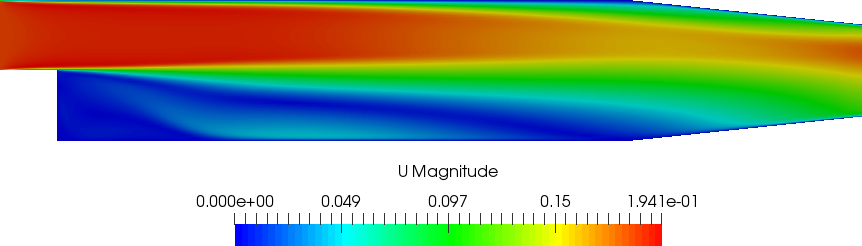
The problems consists of steady Navier-Stokes problem with a parameterized velocity at the inlet. The physical problem is the pitz-daily depicted in the following image
The velocity at the inlet is parameterized in both x and y directions. In other words, the parameters in this setting are the magnitude of the velocity at the inlet and the inclination of the velocity with respect to the inlet.
A detailed look into the code
This section explains the main steps necessary to construct the tutorial N°6.
The necessary header files
First of all let's have a look into the header files which have to be included, indicating what they are responsible for:
The OpenFOAM header files:
#include "fvCFD.H"
#include "fvOptions.H"
#include "IOmanip.H"
#include "simpleControl.H"
ITHACA-FV header files, <ITHACAstream.H> is responsible for reading and exporting the fields and other sorts of data. <ITHACAutilities.H> has the utilities which compute the mass matrices, fields norms, fields error,...etc. <Foam2Eigen.H> is for converting fields and other data from OpenFOAM to Eigen format. <ITHACAPOD.H> is for the computation of the POD modes.
Header file of the Foam2Eigen class.
Header file of the ITHACAPOD class.
Header file of the ITHACAstream class, it contains the implementation of several methods for input ou...
Header file of the ITHACAutilities namespace.
The Eigen library for matrix manipulation and linear and non-linear algebra operations:
#include <Eigen/Dense>
#include <Eigen/SVD>
#include <Eigen/SparseLU>
Header file of the EigenFunctions class.
chrono to compute the speedup
The header files of ITHACA-FV necessary for this tutorial are: <reductionProblem.H> A general class for the implementation of a full order parameterized problem. <steadyNS.H> is for the full order steady NS problem , <SteadyNSTurb.H> is the child of <steadyNS.H> and it is the class for the full order steady NS turbulent problem. Finally <reducedSteadyNS.H> and <ReducedSteadyNSTurb.H> are for the construction of the reduced order problems
Header file of the ReducedSteadyNSTurb class.
Header file of the reducedSteadyNS class.
Header file of the SteadyNSTurb class.
Header file of the reductionProblem class.
Header file of the steadyNS class.
Definition of the tutorial06 class
We define the tutorial06 class as a child of the SteadyNSTurb class. The constructor is defined with members that are the fields required to be manipulated during the resolution of the full order problem using simpleFoam. Such fields are also initialized with the same initial conditions in the solver.
Implementation of a parametrized full order steady turbulent Navier Stokes problem and preparation ...
Class where the tutorial number 6 is implemented.
{
public:
:
{}
autoPtr< volVectorField > _U
Velocity field.
tutorial06(int argc, char *argv[])
Inside the tutorial06 class we define the offlineSolve method according to the specific parameterized problem that needs to be solved. If the offline solve has been previously performed then the method just reads the existing snapshots from the Offline directory, and if the offline solve has been started but not completed then it continues the offline stage from the last snapshot computed. If the procedure has not started at all, the method loops over all the parameters samples, changes the inlet velocity components at the inlet with the iterable parameter sample for both components of the velocity then it performs the offline solve.
void offlineSolve()
Perform an Offline solve.
{
Vector<double> inl(0, 0, 0);
List<scalar> mu_now(2);
{
{
Vector<double>
Uinl(0, 0, 0);
label BCind = 0;
{
}
PtrList< volScalarField > nutFields
List of snapshots for the solution for eddy viscosity.
label counter
Counter used for the output of the full order solutions.
void assignBC(volVectorField &s, label BC_ind, Vector< double > &value)
Assign Boundary Condition to a volVectorField.
bool offline
Boolean variable, it is 1 if the Offline phase has already been computed, else 0.
Eigen::MatrixXd mu
Row matrix of parameters.
void truthSolve()
Perform a TruthSolve.
PtrList< volScalarField > Pfield
List of pointers used to form the pressure snapshots matrix.
PtrList< volVectorField > Ufield
List of pointers used to form the velocity snapshots matrix.
autoPtr< volVectorField > Uinl
Initial dummy field with all Dirichlet boundary conditions.
void read_fields(PtrList< GeometricField< Type, PatchField, GeoMesh > > &Lfield, word Name, fileName casename, int first_snap, int n_snap)
Function to read a list of fields from the name of the field and casename.
else
{
Vector<double>
Uinl(0, 0, 0);
label BCind = 0;
for (label
i = 0;
i <
mu.rows();
i++)
{
}
}
}
This offlineSolve method is just designed to compute the full order solutions for a set of parameters samples called par, the goal is to compute the full order solution for a cross validation test samples which will be used to test the reduced order model in the online stage.
{
Vector<double> inl(0, 0, 0);
List<scalar> mu_now(2);
Vector<double>
Uinl(0, 0, 0);
label BCind = 0;
for (label
i = 0;
i < par.rows();
i++)
{
}
}
{
volScalarField&
p =
_p();
volVectorField&
U =
_U();
IOMRFZoneList& MRF =
_MRF();
#include "NLsolveSteadyNSTurb.H"
}
};
autoPtr< simpleControl > _simple
simpleControl
autoPtr< Time > _runTime
Time.
autoPtr< fvMesh > _mesh
Mesh.
void exportSolution(GeometricField< Type, PatchField, GeoMesh > &s, fileName subfolder, fileName folder, word fieldName)
Export a field to file in a certain folder and subfolder.
simpleControl simple(mesh)
singlePhaseTransportModel & laminarTransport
Definition of the main function
In this section we address the definition of the main function. First we construct the object "example" of type tutorial06:
Then we read the parameters samples for the offline stage and the ones for the online stages using method readMatrix in the ITHACAstream class
word par_offline("./par_offline");
word par_new("./par_online");
List< Eigen::MatrixXd > readMatrix(word folder, word mat_name)
Read a three dimensional matrix from a txt file in Eigen format.
Then we set the inlet boundaries where we have parameterized boundary conditions and we define in which directions we have the parameterization.
example.inletIndex.resize(2, 2);
example.inletIndex(0, 0) = 0;
example.inletIndex(0, 1) = 0;
example.inletIndex(1, 0) = 0;
example.inletIndex(1, 1) = 1;
Then we parse the ITHACAdict file to determine the number of modes to be written out and also the ones to be used for the projection of the velocity, pressure, supremizer and the eddy viscosity:
Class for the definition of some general parameters, the parameters must be defined from the file ITH...
static ITHACAparameters * getInstance()
Gets an instance of ITHACAparameters, to be used if the instance is already existing.
example._runTime());
int NmodesU =
para->ITHACAdict->lookupOrDefault<
int>(
"NmodesU", 5);
int NmodesP =
para->ITHACAdict->lookupOrDefault<
int>(
"NmodesP", 5);
int NmodesSUP =
para->ITHACAdict->lookupOrDefault<
int>(
"NmodesSUP", 5);
int NmodesNUT =
para->ITHACAdict->lookupOrDefault<
int>(
"NmodesNUT", 5);
int NmodesProject =
para->ITHACAdict->lookupOrDefault<
int>(
"NmodesProject", 5);
Now we are ready to perform the offline stage:
The next step is to read the lifting functions
Then we compute the homogeneous velocity field snapshots, and then we output them
example.computeLift(example.Ufield, example.liftfield, example.Uomfield);
void exportFields(PtrList< GeometricField< Type, PatchField, GeoMesh > > &field, word folder, word fieldname)
Function to export a scalar of vector field.
After that, the modes for velocity, pressure and the eddy viscosity are obtained:
void getModes(PtrList< GeometricField< Type, PatchField, GeoMesh > > &snapshots, PtrList< GeometricField< Type, PatchField, GeoMesh > > &modes, word fieldName, bool podex, bool supex, bool sup, label nmodes, bool correctBC)
Computes the bases or reads them for a field.
example.podex,
example.supex, 0, NmodesProject);
example.podex,
example.supex, 0, NmodesProject);
Then we compute the supremizer modes on the basis of the POD pressure modes obtained from the last step
example.solvesupremizer("modes");
then we perform the projection onto the POD modes
example.projectSUP("./Matrices", NmodesU, NmodesP, NmodesSUP,
Now we proceed to the ROM part of the tutorial, at first we construct an object of the class <ReducedSteadyNSTurb.H>.
Now we set the value of the reduced viscosity and we initialize the penalty factor which will be zero
pod_rbf.nu = 1e-3;
pod_rbf.tauU.resize(2, 1);
We create the matrix rbfCoeff in order to store the values of the interpolated eddy viscosity coefficient using the RBF in the online stage
Eigen::MatrixXd rbfCoeff;
Now we solve the online reduced system for the parameter values stored in par_online which is a different set of samples for the parameters than the one used in the offline stage. This represent a cross validation test for assessing the reduced order model in a better way.
for (label k = 0; k < par_online.rows(); k++)
{
Eigen::MatrixXd velNow(2, 1);
velNow(0, 0) = par_online(k, 0);
velNow(1, 0) = par_online(k, 1);
pod_rbf.tauU(0, 0) = 0;
pod_rbf.tauU(1, 0) = 0;
if (stabilization == "supremizer")
{
pod_rbf.solveOnlineSUP(velNow);
}
Now we output the matrix rbfCoeff and the online solution
rbfCoeff.col(k) = pod_rbf.rbfCoeff;
Eigen::MatrixXd tmp_sol(pod_rbf.y.rows() + 1, 1);
tmp_sol(0) = k + 1;
tmp_sol.col(0).tail(pod_rbf.y.rows()) = pod_rbf.y;
pod_rbf.online_solution.append(tmp_sol);
}
"./ITHACAoutput/Matrices/");
"./ITHACAoutput/Matrices/");
"./ITHACAoutput/red_coeff");
"./ITHACAoutput/red_coeff");
void exportMatrix(Eigen::Matrix< T, -1, dim > &matrix, word Name, word type, word folder)
Export the reduced matrices in numpy (type=python), matlab (type=matlab) and txt (type=eigen) format ...
The last step is to reconstruct the velocity and pressure fields using the reduced solution obtained in the online stage and with the POD modes computed earlier on
pod_rbf.reconstruct(true, "./ITHACAoutput/Reconstruction/");
example);
pod_normal.nu = 1e-3;
pod_normal.tauU.resize(2, 1);
for (label k = 0; k < par_online.rows(); k++)
{
Eigen::MatrixXd vel_now(2, 1);
vel_now(0, 0) = par_online(k, 0);
vel_now(1, 0) = par_online(k, 1);
pod_normal.tauU(0, 0) = 0;
pod_normal.tauU(1, 0) = 0;
pod_normal.solveOnline_sup(vel_now);
Eigen::MatrixXd tmp_sol(pod_normal.y.rows() + 1, 1);
tmp_sol(0) = k + 1;
tmp_sol.col(0).tail(pod_normal.y.rows()) = pod_normal.y;
pod_normal.online_solution.append(tmp_sol);
}
"./ITHACAoutput/red_coeffnew");
"./ITHACAoutput/red_coeffnew");
"./ITHACAoutput/red_coeffnew");
pod_normal.reconstruct(true, "./ITHACAoutput/Lam_Rec/");
pod_rbf.uRecFields);
pod_rbf.pRecFields);
pod_rbf.nutRecFields);
"./ITHACAoutput/ErrorsFrob/");
"./ITHACAoutput/ErrorsFrob/");
"./ITHACAoutput/ErrorsFrob/");
pod_rbf.uRecFields);
pod_rbf.pRecFields);
pod_rbf.nutRecFields);
"./ITHACAoutput/ErrorsL2/");
"./ITHACAoutput/ErrorsL2/");
"./ITHACAoutput/ErrorsL2/");
exit(0);
}
Class where it is implemented a reduced problem for the steady Navier-stokes problem.
double errorL2Rel(GeometricField< T, fvPatchField, volMesh > &field1, GeometricField< T, fvPatchField, volMesh > &field2, List< label > *labels)
Computes the relative error between two geometric Fields in L2 norm.
double errorFrobRel(GeometricField< Type, PatchField, GeoMesh > &field1, GeometricField< Type, PatchField, GeoMesh > &field2, List< label > *labels)
Computes the relative error between two Fields in the Frobenius norm.
After we carried out the online stage using an object of the turbulent class <ReducedSteadyNSTurb.H>, now we will repeat same procedure but for the class that does not take into consideration turbulence at the reduced order level which is <reducedSteadyNS.H>. This allows us at the end of comparing the reduced results obtained from both classes.
We finally solve the offline stage for the checking parameters set that was used for validating the reduced order model
#include "fvCFD.H"
#include "fvOptions.H"
#include "IOmanip.H"
#include "simpleControl.H"
#include <Eigen/Dense>
#include <Eigen/SVD>
#include <Eigen/SparseLU>
#include <chrono>
{
public:
:
{}
{
Vector<double> inl(0, 0, 0);
List<scalar> mu_now(2);
{
{
Vector<double>
Uinl(0, 0, 0);
label BCind = 0;
{
}
}
}
else
{
Vector<double>
Uinl(0, 0, 0);
label BCind = 0;
for (label
i = 0;
i <
mu.rows();
i++)
{
}
}
}
{
Vector<double> inl(0, 0, 0);
List<scalar> mu_now(2);
Vector<double>
Uinl(0, 0, 0);
label BCind = 0;
for (label
i = 0;
i < par.rows();
i++)
{
}
}
{
volScalarField&
p =
_p();
volVectorField&
U =
_U();
IOMRFZoneList& MRF =
_MRF();
#include "NLsolveSteadyNSTurb.H"
}
};
int main(
int argc,
char* argv[])
{
word par_offline("./par_offline");
word par_new("./par_online");
example.inletIndex.resize(2, 2);
example.inletIndex(0, 0) = 0;
example.inletIndex(0, 1) = 0;
example.inletIndex(1, 0) = 0;
example.inletIndex(1, 1) = 1;
example._runTime());
int NmodesU =
para->ITHACAdict->lookupOrDefault<
int>(
"NmodesU", 5);
int NmodesP =
para->ITHACAdict->lookupOrDefault<
int>(
"NmodesP", 5);
int NmodesSUP =
para->ITHACAdict->lookupOrDefault<
int>(
"NmodesSUP", 5);
int NmodesNUT =
para->ITHACAdict->lookupOrDefault<
int>(
"NmodesNUT", 5);
int NmodesProject =
para->ITHACAdict->lookupOrDefault<
int>(
"NmodesProject", 5);
word stabilization =
para->ITHACAdict->lookupOrDefault<word>(
"Stabilization",
"supremizer");
example.offlineSolve();
example.computeLift(example.Ufield, example.liftfield, example.Uomfield);
"Uofield");
example.podex,
example.supex, 0, NmodesProject);
example.podex,
example.supex, 0, NmodesProject);
example.podex,
example.supex, 0, NmodesProject);
if (stabilization == "supremizer")
{
example.solvesupremizer("modes");
}
if (stabilization == "supremizer")
{
example.projectSUP("./Matrices", NmodesU, NmodesP, NmodesSUP,
NmodesNUT);
}
else if (stabilization == "PPE")
{
example.projectPPE("./Matrices", NmodesU, NmodesP, NmodesSUP,
NmodesNUT);
}
example);
pod_rbf.nu = 1e-3;
pod_rbf.tauU.resize(2, 1);
Eigen::MatrixXd rbfCoeff;
rbfCoeff.resize(NmodesNUT, par_online.rows());
for (label k = 0; k < par_online.rows(); k++)
{
Eigen::MatrixXd velNow(2, 1);
velNow(0, 0) = par_online(k, 0);
velNow(1, 0) = par_online(k, 1);
pod_rbf.tauU(0, 0) = 0;
pod_rbf.tauU(1, 0) = 0;
if (stabilization == "supremizer")
{
pod_rbf.solveOnlineSUP(velNow);
}
else if (stabilization == "PPE")
{
pod_rbf.solveOnlinePPE(velNow);
}
rbfCoeff.col(k) = pod_rbf.rbfCoeff;
Eigen::MatrixXd tmp_sol(pod_rbf.y.rows() + 1, 1);
tmp_sol(0) = k + 1;
tmp_sol.col(0).tail(pod_rbf.y.rows()) = pod_rbf.y;
pod_rbf.online_solution.append(tmp_sol);
}
"./ITHACAoutput/Matrices/");
"./ITHACAoutput/Matrices/");
"./ITHACAoutput/red_coeff");
"./ITHACAoutput/red_coeff");
"./ITHACAoutput/red_coeff");
pod_rbf.rbfCoeffMat = rbfCoeff;
pod_rbf.reconstruct(true, "./ITHACAoutput/Reconstruction/");
example);
pod_normal.nu = 1e-3;
pod_normal.tauU.resize(2, 1);
for (label k = 0; k < par_online.rows(); k++)
{
Eigen::MatrixXd vel_now(2, 1);
vel_now(0, 0) = par_online(k, 0);
vel_now(1, 0) = par_online(k, 1);
pod_normal.tauU(0, 0) = 0;
pod_normal.tauU(1, 0) = 0;
pod_normal.solveOnline_sup(vel_now);
Eigen::MatrixXd tmp_sol(pod_normal.y.rows() + 1, 1);
tmp_sol(0) = k + 1;
tmp_sol.col(0).tail(pod_normal.y.rows()) = pod_normal.y;
pod_normal.online_solution.append(tmp_sol);
}
"./ITHACAoutput/red_coeffnew");
"./ITHACAoutput/red_coeffnew");
"./ITHACAoutput/red_coeffnew");
pod_normal.reconstruct(true, "./ITHACAoutput/Lam_Rec/");
pod_rbf.uRecFields);
pod_rbf.pRecFields);
pod_rbf.nutRecFields);
"./ITHACAoutput/ErrorsFrob/");
"./ITHACAoutput/ErrorsFrob/");
"./ITHACAoutput/ErrorsFrob/");
pod_rbf.uRecFields);
pod_rbf.pRecFields);
pod_rbf.nutRecFields);
"./ITHACAoutput/ErrorsL2/");
"./ITHACAoutput/ErrorsL2/");
"./ITHACAoutput/ErrorsL2/");
exit(0);
}
Class where it is implemented a reduced problem for the steady turbulent Navier-stokes problem.
autoPtr< volScalarField > _nut
Eddy viscosity field.
autoPtr< surfaceScalarField > _phi
Flux.
autoPtr< fv::options > _fvOptions
fvOptions
autoPtr< singlePhaseTransportModel > _laminarTransport
Laminar transport (used by turbulence model)
autoPtr< IOMRFZoneList > _MRF
MRF variable.
autoPtr< volScalarField > _p
Pressure field.
volVectorField & U
[tutorial06]
 1.13.2